Risk: Measurement, Distributions, and Model Limits
Value at Risk and Stress Tests
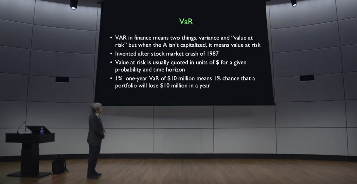
Now I just mentioned there's something else in finance called VAR. Actually, I have on this slide that it means two things. It means variance and it means value at risk. But actually there's a third one that's vector auto regressive, but I was just thinking that it can be confusing. So the variance of a portfolio we've defined is a measure of its variability.
In finance, some people use VAR for value at risk. And this term is relatively new. It didn't appear until after the stock market crash of 1987. And so it's a measure used by some finance people to quantify risk of an investment or of a portfolio. And it's quoted in units of dollars for a given probability and time horizon. So for example, if it says there's a 1% one year value at risk of 10 million.
It means that there's a 1% chance that the portfolio will lose 10 million in one year. And then there's another measure of risk that's become popular in recent years, especially after the financial crisis of 2007 through 9. And that's called a stress test. Now the term stress test goes back to the 1960s or so. And it refers to something that your doctor would order if he was worried about your heart.
And he would have you get on a treadmill in a medical facility and run, and they have an electrocardiarm hooked up to you and they check out your heart while you're under stress, the stress of running. But now the term has moved into finance. So Office of Federal Housing Enterprise Oversight actually was doing stress tests on and Freddie Mac before the 2008 crisis.
Didn't work. Those two firms both failed, but they were trying anyway. So a stress test reflects the idea, it's less, it's not a basic statistical concept, it's a measure, it's a method of assessing risks to firms or portfolios. The idea of the idea of a stress test is that let's look at a portfolio not just by its historical returns and how variable they are, but let's look at the details of the portfolio and ask what vulnerabilities there are for various kinds of financial crises.
Because what actually stresses firms the most are crises. It's not just normal variation. And this is something I'm going to come back to you later in this lecture. that there are extreme events occur. And so the stress test is a test usually ordered by a government to see how some firm will stand up to a financial crisis. So the Dodd-Frank Act in the United States of 2010 requires the Federal Reserve to do annual stress tests for non-bank financial institutions it supervises.
I think they were already doing them for banks. And they want it to be at least three different economic scenarios that the Fed would present. So what they would do is they would get information from the firm about all of their interconnectedness with other institutions, everything they own, how safe is it? And they would look at, say for example, what would happen if there were a severe recession?
Or what would happen if the dollar depreciated or appreciated? Or what would happen if the dollar depreciated? the short-term liquidity crisis where suddenly ability to borrow money at the short-term dries up. The Dodd-Frank Wall Street Reform and Consumer Protection Act was passed into federal law on July 21, 2010, as a response to the financial crisis of 2007 to 2008.
This act constitutes the most significant changes to U.S. financial regulation since the regulatory reform that followed the Great Depression. So the Dodd-Frank Act didn't specify what the three different scenarios were, but they did say that there should be at least three. So this is a different story. This is scenario analysis. It's not something that we're going to emphasize in this course because it's more institutional details that get into the calculations. The European Banking Authority, which was created in 2011 after the financial crisis, has also instituted regular stress tests for European banks.
The United Kingdom, China, and other countries all do stress tests now. But the question is, do they work? Well, there's a growing amount of skepticism that they can really measure what will happen in the next crisis. So Anadmadi is a professor at Stanford who's been arguing, it's all good. garbage. You can't, these guys who are trying to predict what will happen to these companies in a financial crisis, they just don't have the imagination and understanding of how things work out in a panic, in a financial panic. And she thinks that they are just way underestimated.
Generally, the stress tests come out saying it's okay. Don't worry. It does remind me, I was on a stage with the chief economist. of Freddie Mac, here at Yale, we had a, it was around 2005, and he was boasting about their stress tests. And he said that, so I asked him, what about, what if there's a real estate crisis and home prices fall a lot? They were, they were a company that guarantees mortgages on homes.
And so he said, well, we have figured out what would happen to our, portfolio, even under extreme stress situations. So I said, well, what, what is your, I did this on stage, not this stage, it wasn't built yet, but I said, well, what's the, the biggest price decrease you ever considered for your stress test? He said, oh, you know, we considered a 13% drop in home prices.
And then I said to him, well, what if it's bigger than that? And then he looked chagrin. that he said, we've never seen home price drops. Not since the Great Depression. You're not talking about another depression, are you? So we're still friends. I still meet on vacation. But the problem is that home prices fell 30%. Right after that meeting, within a couple of years.
And these two companies, Fannie and Freddie, that were considered safe. Well, actually, if you read the O'Feyo reports on the stress test back then, they'll say, There is some concerns still, you know, they're hedging. But basically they said, don't worry. And then, so that was the end of Ophao, the government shut it down. So the question is whether we can do it this time.
So Anat Admadi doubts that we can do it this time. She thinks there are bigger worries. The stress tests are all coming out. It's no problem, but she's not so sure. If I were CEO of a firm, I imagine I would ask for stress tests. in doing it internally. But you don't want to public, what if it comes out bad? See, the problem is if you ever release that information, then all of your other companies that might do business with you are worried about that.
And so they wouldn't want to do business with you. So it's like your reputation is at stake. So if the government demands that you reveal information for a stress test, you have every incentive to try to whitewash it. And so the question is whether the regulators have enough incentive to demand and push. The Dodd-Frank Act gave regulators the Office of Financial Research subpoena power so they can go in there and demand information from firms.
But it's hard to get it, I think. In the real world, it's a battle. They don't want to tell you.
Understanding Beta through the S&P 500 and Apple
This is the S&P standard and poor 500 stock price index, and it's used as a benchmark for returns. So this is what you did if you just invested in the whole market monthly from 2000 to 2016. And what it shows is a quite a roller coaster ride of value, right? Actually, I should have maybe plotted it longer. It was rising for a long time before that. And then it had a huge drop from a hundred, it fell about in half.
And then starting in 2003, it started a long increase again. And then here's the great financial crisis, 2007 to 2009. And then since that, it's been growing up a lot here. You know, from here to here, this is 2009. From here to here, it tripled in value. It's amazingly unstable, this, stock market to think that the risk of any other company, the law of large numbers is not working here because this is the standard and poor 500 index.
It's an average of 500 stocks. So if they were all independent of each other, the law of large numbers would make the stock market as a whole almost constant. But in fact, it's actually gone up hugely. So there's definite dependence across stock. But I'm not going to be focusing on forecasting the stock market here. We're going to make the assumption that it's very hard to forecast.
So we're going to look at risk as something that we can quantify by looking at the standard deviation of past risks and not focus on what's new right now. what I want to do next is to look at one firm within the S&P 500. What do you think it looks like? If I were to plot Apple, on the same chart here. Did you ever heard anything about how they performed? What's that?
Does anyone know how Apple has performed since 2000? I guess we're not an eager class of stock market devotees. Yes, you didn't, yeah. He said pretty well since the release of the iPhone. And was it 2000? Was it 2007? They did a series of releases of new different models. You're right, they did pretty well. So I'll show you what pretty well means. Now I'm going to superimpose on the same plot, Apple, okay?
That's Apple. It looks different because I had to scale it down to fit Apple onto it. So this is quite a good performance because I've started both, rescale both of them to start it at 100, and it's now at, what is that? $3,500, something like that. So that means a 30, let's say a 40-fold increase in value in 15 years. So imagine that you were taking this class in 2000.
I was teaching this class, that would be 15 years ago. But imagine that you were taking this class then. And you came home to your parents and said, you know, I think Apple stock is a great investment. I just have a quick request of you. Could you take out a second mortgage on the house, borrow $400,000 and put it into Apple stock? Well, if you did that in 2000, your parents would now own over $15 million.
The problem is, what's the problem with that? The problem is nobody knows the future. If you knew that Apple was going to do that, you would have obviously, done this, but nobody knew that Apple was going to do that. So you would also face some problems with your parents if you did that because starting in 2000, Apple dropped quite a bit and you lost, it's like three quarters of your money.
It's hard to tell here, right? It was really limping along for four years. So you come back four years later and your parents said, do you realize what you did? You made us borrow 400,000, and I was just, we're down to 100,000. But then you'd have to be convincing again. No, just hang in there. This is the problem with investing. Hang in there, please. And then it started recovering slowly.
See, I think back then, this was before the iPhone, here back in 2001, two, and three. So it looked like Apple was washed up. When did they bring Steve Jobs back? Do anyone know that? Anyone read about it? I'm assuming you know who Steve Jobs is. Steve Jobs was the founder of Apple Corporation. And he was kind of a difficult guy and kind of quirky. So they fired him.
It was his own company, but you can get fired from your own company. And they put in some professional management, whereas he was kind of a little bit strange. The professional management did this. They brought it down to a low value. And then they invited Steve Jobs back. They thought maybe he does have some kind of genius. But they're still doing well. after his death.
So maybe it's, you know, a company develops a sort of culture and a spree that allows them to keep doing. You know, I really think that's true about organizations. They go on for so long sometimes as a great success. So, for example, the Economist magazine was founded in London in the early 19th century. And it's still a great magazine. How can they last so long?
I went and visited them once and I discovered that they don't even put bylines. They have a different culture. They usually don't put bylines on articles. In other words, if you go to work for The Economist as a writer, you will not become known. They will not put your name, print your name, on the articles you write. So how can they do that? Because young people want to establish themselves somehow.
But they do. And there's a different culture at The Economist magazine as a result. So every company has its own culture and it produces these strange outlier effects. This is the return on Apple stock in red, the red dash line, and the return on the S&P Standard & Poor 500 stock price index. So you can see that the returns on Apple have been very variable, much more variable than the return on the S&P 500.
In fact, when you look at this, it's hard to judge from this picture which one did better, right? It looks like Apple is going up and down all the time. It's this noisy, really noise. And this aggregate stock market looks tamed by comparison. It's hard for you to judge which one did better, but you see it, maybe if you look, you can sort of tell it there are more ups and downs.
But it's so noisy from month to month. These are monthly returns. So here it lost up. Apple lost almost 60% in one month. So it was horrible. The other thing is, I don't know if you can tell that it's correlated with the S&P 500, that when the S&P 500 moves up, it moves up, and when the S&P 500 is down. For example, but see, this is the experience of investing is puzzling because the noise dominates.
It's just so scary watching these things go up. And if you take an interesting investment like Apple, It can, it just goes up and down so much from month to month. And it can look, and it can be under for years, and you can really lose faith in your acumen after it's gone badly for years. So this is just the variance of Apple versus the variance of S&P 500.
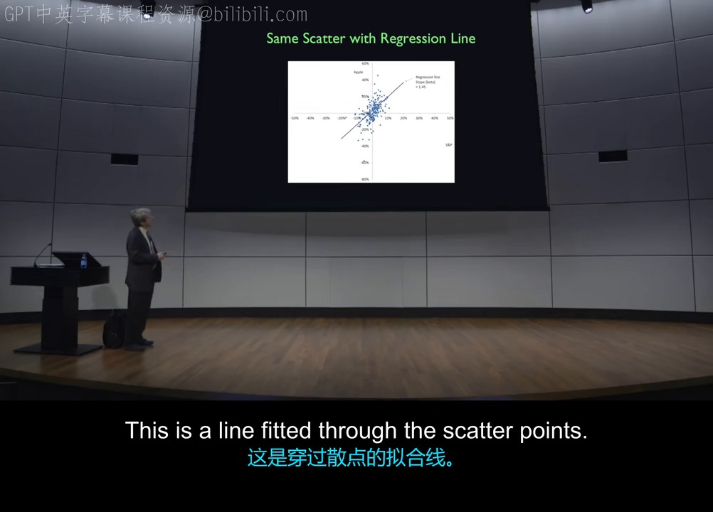
So the standard deviation of Apple capital gain was 12.8 cents a month. That's not annulizing, it means multiplying it by 12. This is a scatter diagram showing the returns on the S&P 500 on the horizontal axis and the returns on Apple on the vertical axis. And you can see that the scatter has an upward slope to it, which means they're correlated. But there's a lot, it's not that strong an upward slope.
But when S&P is high, Apple tends to be high in return. And when S&P is low, Apple tends to be low. But it's more variable. Well, this goes from plus 60 to minus 80. And on this axis, I have minus 50 to plus 50. So it's, Apple is more variable than S&P 500. But you can see that there's a correlation. Actually, it's better if I put a regression line in. This is a line fitted through the scatter of points.
And it shows, it has a slope of 1.45, which is greater than one, which means that Apple overreacts to what happens in the aggregate stock market. And then it has noise on top of that, Apple noise, like Steve Jobs' death noise, that doesn't affect the overall stock market. So Apple actually had, so this is going to be a fundamental concept in this course. The beta of a stock is a measure of how it relates.
to the stock market. If the beta is one, then the asset tends to go up and down one for one in terms of returns with the aggregate market. If the beta is two, they're kind of rare to see beta two stocks. Beta 1.45 is getting high. So Apple reacts more than directly to the stock market. So when times are good, people think they're really good for Apple. And when times are bad, they think it's really bad for Apple.
The concept here is market risk versus idiosyncratic risk. So market risk is the risk of the whole stock market. And for an Apple investment, the market risk of that investment is the risk that Apple will do something in reaction to the aggregate stock market. But idiosyncratic risk is Apple-only risk. So that would be the death of Steve Jobs, or the I-flop.
the iPhone that nobody liked. So they make mistakes. They take risk. The people at Apple have a history of taking risk. They'll try something that might not work out. That's how they, they don't always work out. But on average, they do. So the variance of the return on a stock is equal to its beta squared times the variance of the market return. And that's called systematic risk.
plus the variance of the residual in the regression, the residual in this regression. I think some of this might be, our graduate students can clarify some of these concepts for you. A regression line is a single line that best fits the data in your scatterplot. So how is this calculated? Imagine you have a scatterplot with 50 dots and you start by drawing a line through them.
The vertical distance between a given dot and the regression line is that dot's residual, also known as the error of your proposed line with regards to that single dot. So to get a better fits, I can try changing the slope or constant parameter to force the line to go perfectly through dots 1 and 2, but that'll make the residual associated with dot 3 really big.
So what do we do? We want to minimize some combination of all 50 residuals. So statistics proposes the least squares method. What do the different slopes mean? Remember the equation for a line in algebra class, Y is equal to Mx plus B. The slope M is how much Y changes for a one unit increase in X. In finance, we call Y as the return on Apple stock, X as the return on the market, slope M as beta and the constant B as alpha.
Slope beta tells how much a particular stock co-moves with the market, and thus is a measure of the stock's systematic risk. So the idiosyncratic risk is the risk that the point will lie above or below the line. You can see there's a lot of idiosyncratic risk for Apple.
Normal Distributions, Fat Tails, and Outliers
Now the question is, I was already suggesting that there's an issue of outliers. So what do we mean by an outlier? Well, there's something you've, I'm sure you've heard about, the normal distribution or the bell-shaped curve for random variables. The normal distribution is a typical distribution for random variables in nature. And there are reasons to think that many random variables, follow a distribution like this.
The distribution has two parameters, its mean and its standard deviation. So in this case, I have plotted it for two different standard deviations, but both a mean of zero. So this is a theoretical probability distribution for, let's say, a return on a stock. And here the standard deviation is one on this pink, curve, and it's three on the blue curve. Many random variables in nature follow this distribution, but not all of them.
And that's important because in finance, it tends not to follow this distribution, that we tend to have outliers or fat tails. So this random distribution, the normal distribution, the normal distribution has two tails. This is the right tail, which is high values of the random variable, and here's the left tail, which is low values of the random variable. The height reflects the probability of getting that value.
So if this were the distribution of returns for Apple stock, and let's say standard deviation of three, what, of three, 3%, let's say. Then the probability of getting a return of 3% is pretty good. Well, here's 3%, and the probability of getting three standard deviations out, that would be 9, you can see, is just about negligible. And then I don't even show it anymore.
The probability of 4 standard deviations out is essentially 0. That's what the normal distribution says. Now the normal distribution has been used to describe, for example, human heights or human IQs or SAT scores or lots of things seem to follow the random normal distribution. And you probably have become intuitive about this. If you see some random variable repeatedly and it's always been, you know, pretty much always been between, say, minus 5 and plus 5, then intuitively you start to think it can't happen that it would be 15 because you're intuitively trained by life's experiences.
But in fact, there are other distributions that are more characteristic of financial returns. So there's another kind of distribution called the Koshi distribution, after a famous mathematician. And what I'm showing here is a hundred draws from the normal distribution in blue, and 100. draws from the Koshi distribution in red. Now you see the difference between the Koshi and the normal.
distribution has a kind of look to it. looks, you see, it's going up and down about the same amount all the time. Well, I'm not saying that exactly right. The probability that it would be 10 times the normal change, the usual change, is negligible. So you never see it deviating from, it has a kind of uniform look to it through time. But with Koshi, It also looks very much like normal.
You can't even tell them apart for long intervals of time. And then bang, there's some big positive value. In other words, the distribution under Koshi is fat-tailed. So the Koshi looks like a normal distribution, except instead of just trailing off to zero, the distribution continues out, above zero, way out. So you can be deceived by a fat-tailed distribution like the Koshi into thinking.
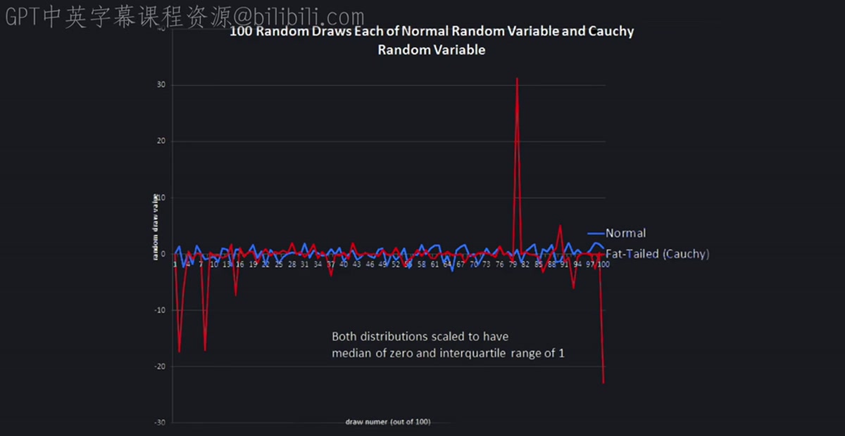
that you're living in a fairly stable world whose risk I understand. But the problem is there are these big events that occur from time to time. The central limit theorem in statistics says that a large, averages of a large number of independent, identically distributed shocks or random variables is approximately normally distributed. But that central limit theorem assumes that the underlying stocks do not have fat tails.
So if you're taking the average of stock market returns, which tend to be fat-tailed, then your average is not a good indication of the real average over long intervals of time. Because you might well have gotten a sample where none of the fat-tailed outlier stocks. So my friend Nassim Taleb has written a book called The Black Swan, which got a lot of attention, referred to Black Swan events.
So you've seen a lot of swans in your lifetime, and they've always been white, right? Have you ever seen a black swan? So you might well conclude that black swans do not exist. But in fact, they do exist. There are black swans. And so that's the metaphor he uses for a fat tail. So here is a plot of the normal and the Koshi distribution. So the Koshi distribution looks pretty much like the normal.
It's a bell-shaped curve. And it trails. off, but there's a subtle difference that there are these rare, very, but they're not quite as rare as the normal would suggest. So the real world puts fat tails in our lives. So here is a plot of the, as a histogram of daily stock price changes since 1928. And what I have, what this thing is, on how many days? there are since 1928, but it's tens of thousands of days.
And so what we're seeing here is that the stock market yield a return of, this is for the S&P 500, or extended S&P 500, of between, I guess this is, between, or of 1% with some interval around that. It did that. On something like 9,500 days, it earned plus 1% on one day. And then on something like 2,500 days, it earned plus 2% percent. And then on something like 800 days it earned plus 3%.
On, what's that? It looks like it's about, I don't know, 400 days it was plus 4%. And then here, I can't you. I can't even figure that out anymore, something at plus 5%. After that, they looked like you can't even see them anymore. So you might conclude by looking at this histogram that stock market returns are always between, say, minus 6% and plus 6%. In matter of fact, on October 30th, 1929, the stock market went up 12.53% in one day.
And on October 19, 1987, the stock market fell 12.53% in one day. fell 20.47% in one day. It was quite a shock. By the way, on this day, I was lecturing, giving my, this class, I was teaching Econ 252. And one of the students was listening to a transistor radio. Do you know what a transistor radio is? It's what they used to have before you had iPhones and things like that.
So he raises, hey, I'd never forget this. And he said, did you know that the stock market is crashing right while you're giving this lecture? So instead of going back to my office, I just thought, what is he saying? I went downtown and I talked to my stockbroker at Merrill Lynch, right here in New Haven. I took the elevator up and just walked in on there just to see what was happening.
And it was this turmoil and everyone. I did manage, because I walked in. If you tried to call your broker, you couldn't. He wouldn't answer. He was too many calls. But I walked in, barged in on him, and I said, what's happening? And he said, don't worry, don't panic. It was this big event, horrible event. But that was the biggest one day drop ever in the whole history of the US stock market.
So I had a good fortune to be warned of it by my student with the transistor radio. The fact that my student, this is before laptops, but he did, we had problems with transistor radios back then. So that's an outlet. So the normal distribution with the same mean in standard deviation as this histogram says that the probability of a drop greater than 20% is equal to 3 times 10 to the minus 71 power.
That's awfully close to zero, if you know. I think that the estimated number of atoms in the universe is bigger. That's 10 to the 80th power. But it's getting on like that. So it's essentially zero. But it's wrong because it happened. And I was there. I saw it happen. And I saw the excitement that it generated.